Aliasing in Computer Graphics
1. Introduction
I’ll keep this intro short and sweet.
I’m picking up where I left off in the last raytracing post: section 7, antialiasing.
2. Aliasing
2.1 Tangent Warning
I first encountered aliasing early in my graphics jouney, as I imagine most do. Drawing anything other than a perfectly vertical or horizontal line tends to result in a visual artifact known coloquially as “jaggies.”
The image below is a zoomed in version of the final output of the last ray tracing post. You can see clearly the aliasing effect at the edge of the sphere.

I’m going to take a little dive into aliasing in this post.
Why? Because, I’m curious. I realized when working through RTIOW that I didn’t understand why it occurs. I knew about it’s visual effect, and I knew a few common techniques for dealing with it, mostly by flipping a switch in OpenGL, but I’d never taken the time to explore the fundamentals surrounding it.
Usually I start to lose sleep when I’m made aware of a gaping hole in my understanding of something. I have a killer urge that pokes at me until I figure it out. So, in the name of a good night’s rest, let’s dig into the fundamentals underlying aliasing in computer graphics.
2.2 Disclaimer
I am by no means in expert in this topic. I simply hope to share some of the intuition I gained in my research and document my learning process. If you’re interested in learning for yourself, check out the sources I’ve linked. They’re awesome; very detailed, and mathematically rigorous.
2.3 The Starting Point
So where can we find the fundamentals that give rise to aliasing?
Enter, Digital Signal Processing (DSP).
2.4 Digital Signal Processing
Computer graphics is really a sub-problem of DSP. There are two primary questions that this field seeks to answer:
- How can we represent continuous data discretely?
- What can we do with that data after it’s been converted it to a digital form?
“It is the mathematics, the algorithms, and the techniques used to manipulate … signals after they have been converted into a digital form” - DSP Chapter 1.
Continuous data usually comes in the form of signals. DSP is dedicated to developing methods to analyze these signals.
So, what’s a signal? Many things… For the most part, it refers to data generated by the real world. Think, “light, sound, seismic vibrations.” DSP provides methods for analyzing these signals in a wide variety of contexts: from space to medical to commercial. But, don’t worry, we don’t need to understand the entire field of DSP to gain insight into why aliasing occurs in computer graphics. In fact, we need only look at one particular step in the DSP pipeline; it just so happens to be probably the most important step in the entire process: Analog-to-Digital Conversion.
Signals (not always, but mostly always) are continuous in nature: “voltage that varies over time; a chemical reaction rate that depends on temperature” - DSP Chapter 3. Before a computer can do any kind of reasoning about a signal, it has to be digitized. In practice this is often done with specialized hardware. Digging into a bit of the mathematics involved in this process can give us the answers we’re looking for as well as a deeper understanding of the graphics pipeline.
Analog-to-Digital Conversion
There are two main steps involved in converting an analog signal to a digital one: sampling and quantization. These processes remove information from the original source, so the name of the game is understanding what information has to be retained and what information can be lost.
Sampling
Sampling is the process of obtaining an instantaneous value of an input signal at periodic intervals - DSP, Chapter 3. It converts the independent variable of a signal from continous to discrete. This is important so I’ll repeat it: Sampling converts the independent variable of a signal from continuous to discrete.
Take a simple example: a sine wave. The formula of the particular wave below is: \(y = 2\sin{(2x)}\)
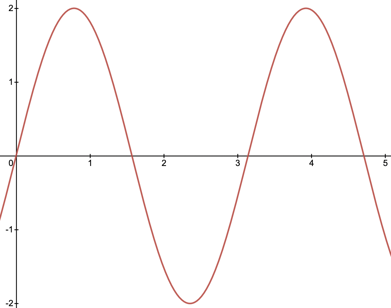
We’ll say the independent variable \(x\) represents some unit of time, and the dependent variable \(y\) represents some measured value. The units for \(x\) and \(y\) could be anything, i.e. amplitude for \(y\), or time in seconds for \(x\). We can keep the units abstract and still understand the idea though.
If we sample the signal at every \(\frac{1}{4} \mathrm{time unit}\), we get the following:
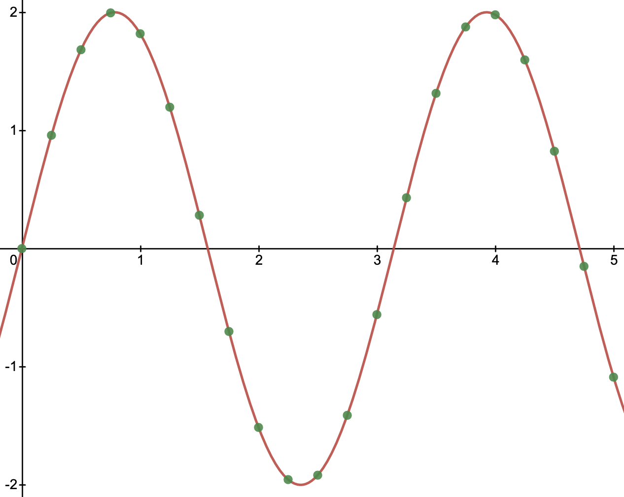
The independent time variable has been converted to discrete (green) points. These points along the wave are our new sampled dataset and all of the values on the wave between points are lost.
There’s an actual circuit that performs this operation called a Sample and Hold Circuit (S/H) - S/H Wiki.
The output of this process becomes the input to the quantization process.
Quantization
So we’ve descritized the independent variable, but the dependent variable is still continuous. It can take on values potentially more precise than a computer can represent. If we had an infinite number of bits to work with than there’d be no need for quantization (or any of this for that matter), but in practice we are always restricted by the capabilities of our hardware. We have to decide on a method to map the continuous dependent variable to a valid integer or float - Aliasing in Computer Graphics. This is quantization.
Quantizing converts a continuous dependent variable into a discrete one.
Quantizing converts a continuous dependent variable into a discrete one.
The Aliasing in Computer Graphics blog and DSP, Chapter 3 have great quantization visualizations.
Proper Sampling
Before moving forward, I’ll warn that I’m going to be even more hand-waving in this section than I already have been. There is a lot of formal mathematics that I’m skipping over. Again, check out the sources if you’re interested.
Despite the fact that both processes remove information from the original signal, in some cases it’s possible to perfectly reconstruct the original analog signal from it’s samples. When this is possble, it’s referred to as proper sampling. “The key information has been captured, and the process can be reversed” - DSP, Chapter 3.
The general idea laid forth in the mathematics is that when sampled properly, there is exactly one signal that could’ve produced a set of samples. Because of that, the process can be reversed to reconstruct the original signal perfectly.
The visual examples here are really great for understanding this. I’ll recreate my own version below.
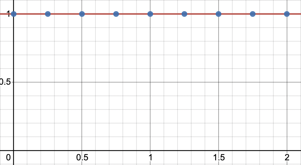
Take, for example, a straight line. It has a frequency of zero, and it’s sampled at every \(\frac{1}{4} \mathrm{time unit}\), the blue points. In this case, it’s clear that the original analog signal can be perfectly reconstructed by connecting the samples with straight line segments.
Now, let’s increase the frequency of the signal, but retain the same samples.
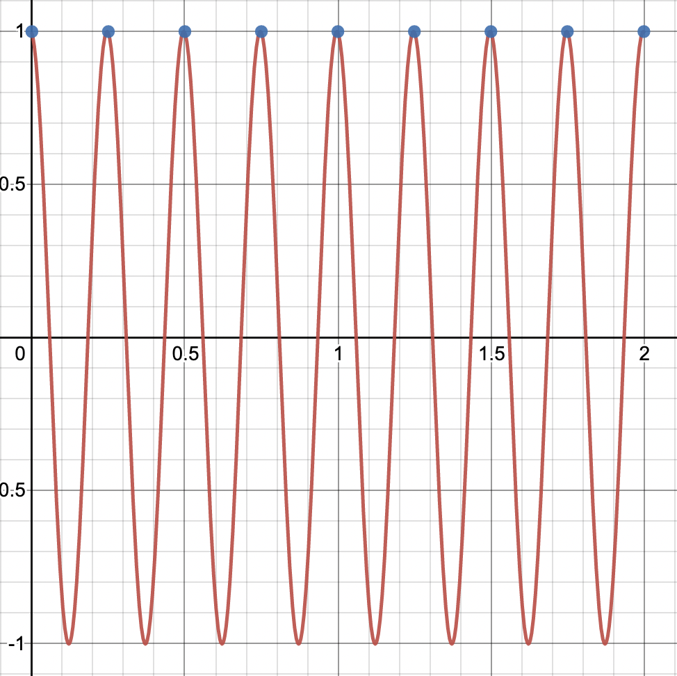
Using the same reconstruction method, straight line segments, will not result in the original signal. An informal way to think about it is that there is “stuff” happening (there’s frequency), between samples. That information is completely lost, and we have no way of knowing that it was ever there. This signal is improperly sampled. In fact, you could say that the signal, when sampled at this rate, assumes a frequency that’s not it’s own - DSP, Chapter 3. It assumes the frequency of a straight line, when it isn’t. It’s true identity is hidden. It has an alias.
Wow… There it is. We made it to the term alias. The logic above describes how we get to something called the Sampling Theorem.
“The sampling theorem indicates that a continuous signal can be properly sampled, only if it does not contain frequency components above one-half of the sampling rate” - DSP, Chapter 3.
There’s a lot more involved in formulating this idea, but hopefully this is enough to start connecting some dots.
Back to Graphics
Okay, how the heck does all of this tie into computer graphics exactly? Well, it turns out, a pixel, the basic building block of graphics, “is not a little square” - A Pixel Is Not A Little Square. A pixel is nothing more than a point sample.
Take the image below.
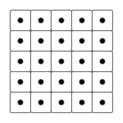
The black dots are the pixels; single point samples. And the squares surrounding each pixel is the reconstruction area.
There are two things happening here:
-
We sample a 2D surface (the viewport) at equidistant points. The specifics of the rendering method will determine what that actually looks like. In ray tracing for example, we’re shooting a ray from the camera’s origin through these point samples and into the scene, checking for intersection with an object to determine a color for that pixel.
-
Now that we have a grid of point samples and we know the color of the image at that point, we can fill the space between the points to reconstruct an image for the viewer. This is where the confusion about what is and isn’t a pixel comes from. In computer graphics we use a box reconstruction filter to fill the color of the screen’s display units (screen “pixels”). The entire display unit takes on the color of the the point sample - A Pixel Is Not A Little Square.
Now let’s see what happens when we place an object in the scene:
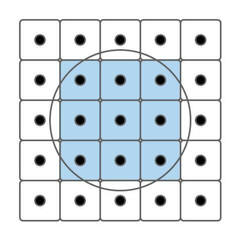
This is an extreme example of course because the resolution is so low. But it shows the effects of aliasing well since the circle ends up being rendered as a square.
Because some of the circle doesn’t overlap pixels (even though it overlaps the reconstruction area), we loose information about its structure. This is like the sine wave graph having frequency between the sample points. Here, there is surface between the sample points.
The Solution
There are many ways to solve this problem, but I’ll look at the method in RTIOW, multi-sampling:
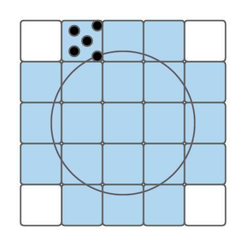
Note: I’m only showing the point samples in one region so the image doesn’t get cluttered.
In multi-sampling, instead of having a single sample per “reconstruction region,” we’ll choose a number of randomly chosen point samples. Then we’ll reconstruct the color of the display unit using the average color of all the sampled points.
Now, of course, there’s still a chance that none of the samples hit the surface of the circle, even if the reconstruction area does. Adding more samples reduces this chance, but also increases rendering time, so there’s a trade off.
3. Last Words
It’s interesting what you can learn when you entertain a small tangent. I started this post wanting to learn a bit more about the causes of aliasing, and I came away with a better understanding of Digital Signal Processing, Sampling, Quantization, and an entirely new understanding of what a pixel is.
Below are the results of multi-sampling. The image on the left is rendered using single samples and the image on the right is using 300 samples per pixel.