• 1. Intro
  • 1.1 The Purpose of this Post
  • 1.2 Ray Tracing in One Weekend
• 2. Ray Tracing Basics
  • 2.1 The Ray, the Scene, and the Camera
  • 2.2 The Ray
  • 2.3 The Screen
  • 2.4 Camera
  • 2.5 Objects
    • 2.5.1 Ray-Sphere Intersection
    • 2.5.2 Note: Accounting for Z
• 3. Normals
  • 3.1 Sphere Normals
  • 3.2 Front Faces/Back Faces
• 4. A Sphere
• 5. Sources

1. Intro

1.1 The Purpose of this Post

This is the first post in a series where I’ll document my progress learning the ins and outs of ray tracing.

My short term goal is simply to learn more about ray tracing because I’m curious. I’ll start by working through each of the books in the RTIOW¹ series. My long term (maybe overly ambitious) goal is to develop a real-time ray tracing graphics engine for game development. The focus right now though is on working through the basics, real-time ray tracing and hardcore optimizations can come later when I gain a better sense of the basic features and existing standard optimization approaches.

For now these posts will take the form of notes I’m taking on the sources I’m reading. RTIOW will be the main guide to get all of the basic features implemented. I’m also reading through some of the papers in the first volume of Ray Tracing Gems², so there may be tangents to summarize what I’m learning there.

Without further ado…

1.2 Ray Tracing in One Weekend

Ray Tracing in One Weekend is a tutorial written by Peter Shirley, a Computer Scientist with a serious amount of experience in computer graphics. The goal of the series is to, as quickly as possible, guide the reader through the development of the major features of a ray tracer. It is extremely well crafted and informative. If you have any interest in Ray Tracing definitely check it out here.

2. Ray Tracing Basics

2.1 The Ray, the Scene, and the Camera

What is a ray tracing?

• A rendering technique that produces images by intersecting rays with objects and computing the pixel color based on that intersection.

The most basic components of a ray tracer:

• Ray
• Screen
• Camera (a method to define the angle at which the ray passes through the pixel)
• Object

The Steps:

1. Calculate the ray from the eye to the pixel
2. Determine which objects the ray intersects
3. Compute a color for the intersection point

2.2 The Ray

The ray is the most fundamental structure in a ray tracer. It refers to a three dimensional half line usually specified as an interval on a line². In two dimensions a line can be defined by it’s implicit form \(y = mx + b\). Interestingly, though there is no implicit formula for a line in three dimensions, so the parametric form is used:

\(\mathbf{P}(t) = (1 - t)\mathbf{A} + t\mathbf{B}\).

In this function, \(\mathbf{A}\) and \(\mathbf{B}\) are any two points, so \(\mathbf{P}(t)\) becomes the weighted average between those two points. If we interpret \(\mathbf{A}\) as the ray’s origin and \(\mathbf{B}\) as the ray’s direction then we can rewrite the ray function as:

• \(\mathbf{P}\) : a point along a line in 3D space (vector)
• \(\mathbf{A}\) : the ray origin (vector)
• \(\mathbf{b}\) : the ray direction (vector)
• \(t\) : a parameter (real number)
  • \(t\) moves \(\mathbf{P}\) along the ray
  • The sign of \(t\) determines whether \(\mathbf{P}\) is in front of or behind of \(\mathbf{A}\)

In code a basic ray structure may look something like this:

struct Ray
{
   Vec3 Origin;
   Vec3 Direction;
	
   Vec3 At(double t)
   {
      return Origin + t * Direction;
   }
};

2.3 The Screen

For now the ray tracer doesn’t produce interactive scenes. It renders a single frame to a buffer, and then converts the buffer to an image file in the PPM Image File Format³. I probably won’t use the PPM Format for too long so I won’t spend a lot of time on it here.

2.4 Camera

The picture from RTIOW works well to describe the relationship between the camera, the ray and the view port. The image below is from the book¹.

Some important things to note about the camera setup shown in the picture:

• +X: right, +Y: up, -Z: into the screen
  
• The ray tracer traverses the view port from the upper left hand corner, using two offset vectors (\(\mathbf{u}\), \(\mathbf{v}\)) to move the ray endpoint
  
• Pixel index [0][0] is at the lower-left corner of the view port
  

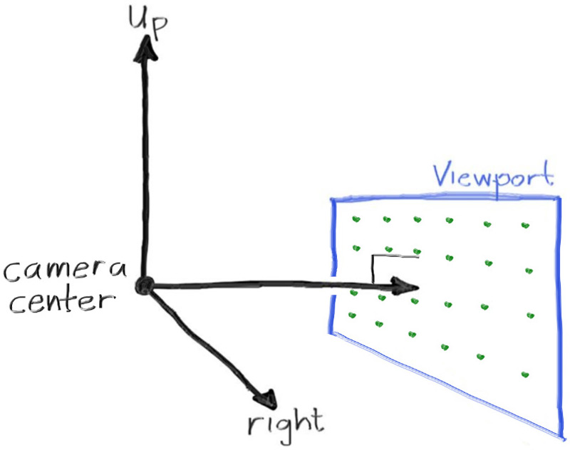
Here’s the math to describe the camera, view port and ray in the image above.

Let the:
image width in pixels be \(w\),
image height in pixels be \(h\),
aspect ratio be \(ar = w / h\),
view port height be \(vh = 2\),
view port width be \(vw = ar \cdot vh\),
focal length be \(fl = 1\),
eye position be \(\mathbf{e} = \mathbf{0}\).

The horizontal vector can be defined as \(\mathbf{horizontal} = (vw, 0, 0)\).
The vertical vector can be defined as \(\mathbf{vertical} = (0, vh, 0)\).
The lower left corner point can be defined as \(\mathbf{l} = \mathbf{e} - \mathbf{h} / 2 - \mathbf{v} / 2 - (0, 0, fl)\).

Then \(\mathbf{u}\) and \(\mathbf{v}\) can be defined as:

where \(i\) goes from 0 to (\(w\) - 1) and \(j\) goes from (\(h\) - 1) to 0.

Note:
	- v (starts at 1 and goes to 0)
	- u (starts at 0 and goes to 1)

The ray direction can finally be calculated:

\(\mathbf{dir} = \mathbf{l} + u \cdot \mathbf{h} + v \cdot \mathbf{v} - \mathbf{e}\).

The code for the initialization of a ray at pixel location \((i, j)\) looks like this:

for (int i = 0; i < imageHeight; i++)
{
   for (int j = 0; j < imageWidth; j++)
   {
      double u = (double) j / (double)(imageWidth - 1);
      double v = (double)(imageHeight - i - 1) / (double)(imageHeight - 1);
      
      Ray r(origin, 
            lowerLeftCorner + u * horizontal + v * vertical - origin);
      ...
   }
}

2.5 Objects

A pixel’s color is derived from the object(s) that it overlaps with along the ray’s trajectory into the scene. Without objects for the ray to collide with, there will be nothing to color the pixels. For now spheres are the only supported geometry, but I’m writing the code so that it can be extended relatively easy. It looks something like this:

struct HittableSphere
{
   Vec3 Center;
   double Radius;

   bool Hit(...);
};

enum class HittableType
{
   SPHERE,
   ...
};

struct Hittable
{
   HittableType Type

   union
   {
      HittableSphere Sphere;
      ...
   };

   bool Hit(...);
};

The pattern above is referred to as a tagged union. The Hit function in the Hittable struct simply checks Type with a switch statement and calls the Hit function on the appropriate union data member. Another solution to this problem is to make Hittable an abstract base class and then specific geometries like a sphere or cube would derive from it and provide an implementation of the hit function. The reason I’m not doing it that way is simply personal preference. I tend to write C++ in a more C style way, avoiding higher level language constructs unless there is a very clear reason not to.

2.5.1 Ray-Sphere Intersection

The equation of a sphere centered around the origin with radius \(R\):

\(x^2 + y^2 + z^2 = R^2\).

The interpretation of equality for point (x, y, z):

• ON sphere surface: \(x^2 + y^2 + z^2 = R^2\)
• INSIDE sphere: \(x^2 + y^2 + z^2 < R^2\)
• OUTSIDE sphere: \(x^2 + y^2 + z^2 > R^2\)

The equation of a sphere centered around \((Cx, Cy, Cz)\):

To write the above in terms of vectors, let \(\mathbf{C} = (Cx, Cy, Cz)\), and \(\mathbf{P} = (x, y, z)\).

Then,

And finally,

Any point that satisfies the last equation is on the surface of the sphere. The ultimate question we are trying to answer here is: does a ray \(\mathbf{P}(t) = \mathbf{A} + t\mathbf{b}\) intersect the sphere? Does it intersect at one point, two points or no points? If it does intersect, what is \(t\) that satisfies the sphere equation?

To answer this lets first substitute the ray equation for \(\mathbf{P}\):

Then, expand and move all terms to the left to get the final equation for ray-sphere intersection:

This is a quadratic equation with one unknown \(t\) and can be solved using the good ole quadratic equation:

\(t = \frac {-b \pm \sqrt {b^2 - 4ac}}{2a}\).

The discriminant describes the nature of the intersection:

• Positive - two real solutions: hit
• Zero - one real solution: hit
• Negative - no real solutions miss

Solving the equation will give us the \(t\) value of the intersection which can be used to compute the point of intersection \(\mathbf{P}\).

The components of the quadratic equation can be defined as:
\(a = b\cdot b\)
\(b = 2\mathbf{b} \cdot (\mathbf{A} - \mathbf{C})\)
\(c = (\mathbf{A} - \mathbf{C}) \cdot (\mathbf{A} - \mathbf{C}) - r^2\)

Finally, a simple function to check if a ray intersects a sphere:

bool HitSphere(const Vec3& center, double radius, const Ray& ray)
{
	Vec3 oc = ray.Origin - center;
	double a = Dot(ray.Direction, ray.Direction);
	double b = 2.0f * Doc(oc, ray.Direction);
	double c = Dot(oc, oc) - radius * radius;
	double discriminant = b * b - 4 * a * c;
	return discriminant > 0;
}

2.5.2 Note: Accounting for Z

The ray-sphere intersection described so far will produce the same output whether the object is in front of the camera (\(-z\)), or behind the camera (\(+z\)). This is because there’s no consideration of the sign of \(t\) at the intersection point. Recall that positive values of \(t\) will produces points in front of the camera while negative values of \(t\) will produce points behind the camera. Setting a min and a max for \(t\) becomes useful for solving several problems, this is one of them.

3. Normals

3.1 Sphere Normals

The outward normal for a sphere is simply the hit point minus the center: \(\mathbf{P} - \mathbf{C}\)

3.2 Front Faces/Back Faces

There are two kinds of normals: front face and back face. Front facing normals point out from the surface of the object while back facing normals point into the surface of the object. Both are useful and will be generated based on the ray direction. We want a front facing normal when the ray hits from outside the object and a back facing normal when the ray hits from inside an object. This means we always produce a normal that points against the direction of the ray. So for ray \(\mathbf{r}\) and normal \(\mathbf{n}\):

I like the hit function above because it’s a good reminder of how simple the most basic concept of ray tracing really is. Already though, it’s clear that there are many nuances to consider in a real ray tracer. Here is the first extension of the hit function to address the \(z\) and normals issues I mentioned above.

struct HitRecord
{
   Vec3 Point;
   Vec3 Normal;
   bool FrontFaceNormal;
   double T;
   
   void SetNormal(const Ray& ray, const Vec3& frontFaceNormal)
   {
      if (Dot(ray.Dir, frontFaceNormal) > 0.0f)
      {
         // ray and normal facing in same direction
         // means ray is coming from inside the object
         Normal = -frontFaceNormal;
         FrontFaceNormal = false;
      }
      else
      {
         // ray and normal facing in opposite directions
         // means ray is coming from outside the object
         Normal = frontFaceNormal;
         FrontFaceNormal = true;
      }
   }
};

bool HitSphere
(
   const Vec3& center, 
   double radius, 
   const Ray& ray,
   double tMin,
   double tMax,
   HitRecord& record
)
{
   // Calculate a, b, c and the discriminant
   Vec3 o_minus_c = ray.Origin - center;
   double a = Dot(ray.Direction, ray.Direction);
   double b = 2.0f * Doc(o_minus_c, ray.Direction);
   double c = Dot(o_minus_c, o_minus_c) - radius * radius;
   double discriminant = b * b - 4 * a * c;
	
   if (discriminant < 0) return false;

   // Find closest t in range (tMin, tMax)
   double sqrt_d = sqrt(discriminant);
   double root = (-b - sqrt_d) / (2 * a);
   if (root < tMin || root > tMax)
   {
      root = (-b + sqrt_d) / (2 * a);
      if (root < tMin || root > tMax)
         return false;
   }

   // Fill out hit record
   record.T = root;
   record.Point = ray.At(root);
	
   Vec3 front_face_normal = (record.Point - center) / radius;
   record.SetNormal(ray, front_face_normal);

   return true;
}

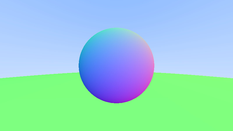
4. A Sphere

Here’s an image of the output so far. There is a gradient background and two spheres. The color’s are derived from the surface normals like this:

...
Vec3 color = 0.5 * (record.Normal + Vec3(1.0f, 1.0f, 1.0f));
...

5. Sources